Understanding Modern RAG: Retrieval, Generation, and Everything Between
You’ve probably heard that Retrieval-Augmented Generation (RAG) is the secret sauce behind smarter AI applications. But what actually happens when you ask a RAG system a question? And more importantly, how do you build one that doesn’t hallucinate or miss obvious answers? In this tutorial, you’ll learn the core components of modern RAG systems—from chunking strategies to embedding models to generation—with concrete code examples you can run today. We’ll demystify vector databases, retrieval mechanisms, prompt construction, and evaluation metrics. By the end, you’ll understand not just what RAG is, but how each piece fits together and why certain design choices matter.
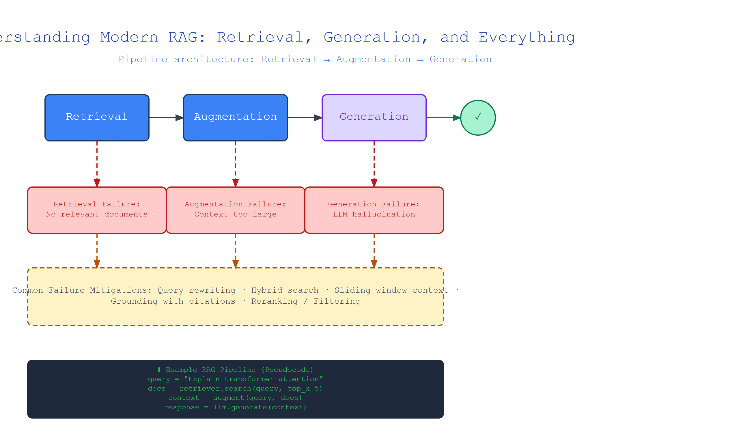
The Foundation: What Is Retrieval-Augmented Generation?
Plain-English definition: RAG is a technique where an AI model searches a knowledge base for relevant information before generating an answer. Think of it like giving a student open-book exam instructions instead of forcing them to memorize everything.
How it works under the hood: When a user asks a question, the system first converts that question into a numerical representation (a vector embedding). It then searches a pre-indexed database of document chunks for the most similar vectors. The top results are retrieved and inserted into a prompt before being sent to a large language model (LLM) for generation.
Real-world analogy: Imagine you’re a librarian. A patron asks “What’s the capital of France?” Instead of reciting from memory (pure generation), you walk to the reference section, pull the atlas (your vector database), find the relevant page (retrieval), and then read the answer aloud (generation).
Annotated code snippet:
# Simple RAG pipeline using LangChain and OpenAI
from langchain.document_loaders import TextLoader
from langchain.text_splitter import RecursiveCharacterTextSplitter
from langchain.embeddings import OpenAIEmbeddings
from langchain.vectorstores import Chroma
from langchain.llms import OpenAI

# Step 1: Load and chunk your documents
loader = TextLoader("company_policy.txt")
documents = loader.load()
text_splitter = RecursiveCharacterTextSplitter(chunk_size=500, chunk_overlap=50)
chunks = text_splitter.split_documents(documents)

# Step 2: Create embeddings and store in vector database
embeddings = OpenAIEmbeddings()
vectorstore = Chroma.from_documents(chunks, embeddings)

# Step 3: Set up retriever and LLM
retriever = vectorstore.as_retriever(search_kwargs={"k": 3})
llm = OpenAI(temperature=0)

# Step 4: Query with retrieval
def ask_rag(query):
    docs = retriever.get_relevant_documents(query)
    context = "\n".join([doc.page_content for doc in docs])
    prompt = f"Based on the following context, answer the question.\n\nContext: {context}\n\nQuestion: {query}"
    return llm(prompt)

print(ask_rag("What is our vacation policy?"))
Non-obvious insight: Chunk overlap is critical. Without it, a sentence split across two chunks will be lost—your model will answer confidently with incomplete information.
Vector Embeddings: Turning Words into Math
Plain-English definition: A vector embedding is a list of numbers (usually 300-1500 of them) that represents the meaning of a piece of text. Similar meanings produce similar numbers.
How it works under the hood: A neural network trained on billions of text pairs learns to map words and phrases to positions in a high-dimensional space. Words like “king” and “queen” end up closer to each other than “king” and “apple.” The actual numbers come from the network’s internal calculations—you don’t manually assign them.
Real-world analogy: Think of each document as a point on a giant map. Dog-related documents cluster together near “dog park,” while cooking documents sit near “kitchen.” The embedding model figures out where each document belongs on this map.
Annotated code snippet:
from sentence_transformers import SentenceTransformer
import numpy as np

model = SentenceTransformer('all-MiniLM-L6-v2')

# Example sentences
sentences = [
    "The cat sat on the mat",
    "A feline rested on the rug",
    "I like to eat pizza"
]

# Generate embeddings (each is a 384-dimensional vector)
embeddings = model.encode(sentences)
print(f"Embedding shape: {embeddings.shape}")  # (3, 384)

# Check similarity between first two sentences (similar meaning)
cosine_sim_1_2 = np.dot(embeddings[0], embeddings[1])
print(f"Similarity 'cat' vs 'feline': {cosine_sim_1_2:.3f}")  # ~0.85

# Check similarity between first and third (unrelated)
cosine_sim_1_3 = np.dot(embeddings[0], embeddings[2])
print(f"Similarity 'cat' vs 'pizza': {cosine_sim_1_3:.3f}")  # ~0.20
Non-obvious insight: Most people use general-purpose embedding models for specialized domains. If your dataset is medical or legal, train or fine-tune a domain-specific embedding model—the difference in retrieval accuracy is often 15-30%.
Vector Databases: The Search Engine for Meanings
Plain-English definition: A vector database is a specialized storage system that can instantly find the most similar items to a query vector, rather than matching exact keywords.
How it works under the hood: Instead of using B-tree indexes like traditional databases, vector databases use approximate nearest neighbor (ANN) algorithms like HNSW (Hierarchical Navigable Small World) or IVF (Inverted File Index). These create multi-layer graph structures that let you jump to the right neighborhood quickly, then search locally.
Real-world analogy: If you’re looking for a friend in a stadium, a vector database doesn’t check every seat (brute force). It first asks “which section?” then “which row?” then “which seat?”—the hierarchical approach makes it fast even with millions of items.
Annotated code snippet using Pinecone:
import pinecone

# Initialize connection
pinecone.init(api_key="your-api-key", environment="us-west1-gcp")

# Create index with proper dimensions
index_name = "company-docs"
if index_name not in pinecone.list_indexes():
    pinecone.create_index(
        name=index_name,
        dimension=384,  # Must match your embedding model's output
        metric="cosine"
    )

index = pinecone.Index(index_name)

# Insert vectors with metadata
vectors_to_insert = [
    ("id-1", embedding_1.tolist(), {"title": "Vacation Policy", "date": "2024-01-15"}),
    ("id-2", embedding_2.tolist(), {"title": "Health Benefits", "date": "2024-02-01"})
]
index.upsert(vectors=vectors_to_insert)

# Query with filters
query_results = index.query(
    vector=query_embedding.tolist(),
    filter={"date": {"$gte": "2024-01-01"}},
    top_k=5,
    include_metadata=True
)
Non-obvious gotcha: Vector databases don’t handle updates well. If you change a single document, you must re-embed and re-insert that chunk. This is why versioned indices and periodic rebuilds are common in production.
Retrieval Strategies: Not All Searches Are Created Equal
Plain-English definition: The retrieval stage decides which documents to pull from the database. Different strategies balance relevance, speed, and diversity.
Key mechanisms:
- Similarity search: Returns the most similar vectors by cosine distance
- Maximum marginal relevance (MMR): Similarity + diversity—penalizes results that are too similar to each other
- Hybrid search: Combines vector similarity with keyword matching (BM25) for better recall
- Multi-query retrieval: Generates multiple query variations to cast a wider net
Real-world analogy: Similarity search is like asking one friend for restaurant recommendations. MMR is like asking three friends from different social circles—more diverse picks. Hybrid search is combining Yelp ratings with menu keywords.
Annotated code snippet showing MMR:
from langchain.vectorstores import Chroma

# Setup with MMR retriever
vectorstore = Chroma.from_documents(all_chunks, embeddings)
retriever = vectorstore.as_retriever(
    search_type="mmr",
    search_kwargs={
        "k": 5,
        "fetch_k": 20,  # Fetch more then filter for diversity
        "lambda_mult": 0.5  # 0 = pure diversity, 1 = pure similarity
    }
)

# Compare results
similar_results = vectorstore.similarity_search("vacation policy", k=5)
mmr_results = retriever.get_relevant_documents("vacation policy")

print(f"Similarity results: {[d.metadata['section'] for d in similar_results]}")
print(f"MMR results: {[d.metadata['section'] for d in mmr_results]}")
Non-obvious insight: MMR is critical when your documents are repetitive (like FAQs). Without it, you’ll get 5 nearly identical chunks instead of covering different aspects of the topic.
Evaluation: Is Your RAG System Actually Working?
Plain-English definition: Evaluation measures how well your RAG system retrieves relevant documents and generates accurate answers.
Key metrics:
- Hit rate: Percentage of queries where at least one relevant document is retrieved
- Mean Reciprocal Rank (MRR): How high the first relevant result appears (1 = first, 0.5 = second)
- Answer faithfulness: Does the generated answer contradict the retrieved context?
- Answer relevance: Does the answer actually address the question?
Code example using RAGAS evaluation:
from ragas import evaluate
from ragas.metrics import faithfulness, answer_relevancy
from datasets import Dataset

# Prepare your evaluation data
eval_data = Dataset.from_dict({
    "question": ["What is the vacation policy?", "How many sick days?"],
    "answer": ["Three weeks per year.", "Ten sick days annually."],
    "contexts": [
        [vacation_doc.page_content],
        [sick_leave_doc.page_content]
    ],
    "ground_truth": ["3 weeks paid vacation", "10 sick days per year"]
})

# Compute metrics
result = evaluate(
    eval_data,
    metrics=[faithfulness, answer_relevancy]
)
print(f"Faithfulness: {result['faithfulness']:.2f}")
print(f"Relevancy: {result['answer_relevancy']:.2f}")
Non-obvious insight: Most teams optimize for retrieval accuracy but forget to check whether the LLM actually uses the retrieved context. A common failure mode: the LLM ignores the context entirely and hallucinates based on its training data.
Comparison Table: RAG Components at a Glance
| Component | What It Does | Key Metric | Common Pitfall |
|---|---|---|---|
| Chunking | Splits documents into searchable pieces | Chunk size & overlap | Splitting in the middle of sentences |
| Embeddings | Converts text to numerical vectors | Cosine similarity | Using wrong model for your domain |
| Vector DB | Stores and searches embeddings | Query latency | Ignoring metadata filtering |
| Retriever | Fetches relevant chunks | Hit rate @ k | Forgetting diversity (MMR) |
| Generator | Produces final answer | Answer faithfulness | LLM ignoring retrieved context |
Key Takeaways
- RAG combines retrieval and generation — think of it as an open-book exam for AI models
- Chunking strategy matters more than most people think; 500-1000 tokens with 10-20% overlap is a good starting point
- Embeddings map meaning to numbers — choose or fine-tune models for your specific domain
- Vector databases enable efficient similarity search using ANN algorithms, not brute force
- Retrieval strategies like MMR improve answer diversity and coverage
- Evaluation isn’t optional — always measure both retrieval accuracy and answer faithfulness
- Context quality beats context quantity — five great chunks outperform twenty mediocre ones

Comments